Take-home Exercise 3
1 Introduction
Around 77.9% of dwellings in Singapore are made up of Housing and Development Board (HDB) flats, public housing many residents are familiar with and take pride in.
Though the number of households living in HDB apartments continues to increase, there is a steady fall in number of Singaporeans actually living in these flats. One argument provided is that more Singaporeans are selling their flats and “upgrading” to private housings, like condominium and private landed properties. Among those upgrading, selling their current house to afford for a better HDB apartments is not uncommon too.
On the flip side, there is the demand and there are many reasons for residents to buy resale flats.
- Families may not be keen to wait approximately 2 to 5.9 years for an apartment under the Build-to-Order exercise.
- Couples, being both Permanent Residents, can only access the resale market, if they want to buy a HDB flat.
- Single citizens similarly are only allowed to purchase resale flats.
In spite of the ever increasing resale prices, increasing 8.7% YoY, and much more expensive than a BTO flat, resale flats continue to be in the cards for residents to buy their dream homes.
With how expensive these apartments are, you better bet that people will be choosing where to place their money more carefully.
With 3-room flats having a more diverse demographics of buyers, I would like to focus on this particular flat type in this exercise.
2 Import Packages
Below the packages that we will be using in this exercise:
3 Import Data
| Dataset | Source |
|---|---|
| HDB Resale Flat Prices | Data.gov.sg |
| Masterplan 2019 Subzone Boundary | Professor Kam Tin Seong |
| Hawker Centres | OpenMapSG |
| Elderly Centres | OpenMapSG |
| Parks | OpenMapSG |
| Kindergartens | OpenMapSG |
| Childcare Centres | OpenMapSG |
| Bus Stops | LTA DataMall |
| MRT Stations | LTA DataMall |
| Primary Schools | OpenMapSG |
| Supermarkets | OpenMapSG |
| Malls | Wikipedia |
| HDB MUP/HIP Status | Housing Development Board |
3.1 Import HDB Resale Flat Prices
# A tibble: 5 × 11
month town flat_…¹ block stree…² store…³ floor…⁴ flat_…⁵ lease…⁶ remai…⁷
<chr> <chr> <chr> <chr> <chr> <chr> <dbl> <chr> <dbl> <chr>
1 2017-01 ANG MO … 2 ROOM 406 ANG MO… 10 TO … 44 Improv… 1979 61 yea…
2 2017-01 ANG MO … 3 ROOM 108 ANG MO… 01 TO … 67 New Ge… 1978 60 yea…
3 2017-01 ANG MO … 3 ROOM 602 ANG MO… 01 TO … 67 New Ge… 1980 62 yea…
4 2017-01 ANG MO … 3 ROOM 465 ANG MO… 04 TO … 68 New Ge… 1980 62 yea…
5 2017-01 ANG MO … 3 ROOM 601 ANG MO… 01 TO … 67 New Ge… 1980 62 yea…
# … with 1 more variable: resale_price <dbl>, and abbreviated variable names
# ¹flat_type, ²street_name, ³storey_range, ⁴floor_area_sqm, ⁵flat_model,
# ⁶lease_commence_date, ⁷remaining_lease3.1.0.1 Convert “Month” to DataTime Format
As we want to have the abilities to filter the data according to its dates, it’s best for us to convert the date column to a DateTime format.
3.1.0.1.1 Data - Filter Jan 2021 to Feb 2023
Here, we will filter the data so we will only be working with those from January 2021 to February 2023.
# A tibble: 5 × 12
month town flat_…¹ block stree…² store…³ floor…⁴ flat_…⁵ lease…⁶ remai…⁷
<chr> <chr> <chr> <chr> <chr> <chr> <dbl> <chr> <dbl> <chr>
1 2021-01 ANG MO … 2 ROOM 170 ANG MO… 01 TO … 45 Improv… 1986 64 yea…
2 2021-01 ANG MO … 2 ROOM 170 ANG MO… 07 TO … 45 Improv… 1986 64 yea…
3 2021-01 ANG MO … 3 ROOM 331 ANG MO… 04 TO … 68 New Ge… 1981 59 yea…
4 2021-01 ANG MO … 3 ROOM 534 ANG MO… 04 TO … 68 New Ge… 1980 58 yea…
5 2021-01 ANG MO … 3 ROOM 561 ANG MO… 01 TO … 68 New Ge… 1980 58 yea…
# … with 2 more variables: resale_price <dbl>, date <date>, and abbreviated
# variable names ¹flat_type, ²street_name, ³storey_range, ⁴floor_area_sqm,
# ⁵flat_model, ⁶lease_commence_date, ⁷remaining_lease3.2 Import Subzone Data
subzone_sf <- st_read(dsn="data/geospatial/MPSZ-2019", layer="MPSZ-2019") %>% st_transform(crs = 3414)Reading layer `MPSZ-2019' from data source
`C:\deadline2359\IS415-GAA\Take-home_Ex\Take-home_Ex03\data\geospatial\MPSZ-2019'
using driver `ESRI Shapefile'
Simple feature collection with 332 features and 6 fields
Geometry type: MULTIPOLYGON
Dimension: XY
Bounding box: xmin: 103.6057 ymin: 1.158699 xmax: 104.0885 ymax: 1.470775
Geodetic CRS: WGS 84Simple feature collection with 6 features and 6 fields
Geometry type: MULTIPOLYGON
Dimension: XY
Bounding box: xmin: 8012.578 ymin: 22108.68 xmax: 35287.9 ymax: 31092.38
Projected CRS: SVY21 / Singapore TM
SUBZONE_N SUBZONE_C PLN_AREA_N PLN_AREA_C REGION_N
1 MARINA EAST MESZ01 MARINA EAST ME CENTRAL REGION
2 INSTITUTION HILL RVSZ05 RIVER VALLEY RV CENTRAL REGION
3 ROBERTSON QUAY SRSZ01 SINGAPORE RIVER SR CENTRAL REGION
4 JURONG ISLAND AND BUKOM WISZ01 WESTERN ISLANDS WI WEST REGION
5 FORT CANNING MUSZ02 MUSEUM MU CENTRAL REGION
6 MARINA EAST (MP) MPSZ05 MARINE PARADE MP CENTRAL REGION
REGION_C geometry
1 CR MULTIPOLYGON (((33222.98 29...
2 CR MULTIPOLYGON (((28481.45 30...
3 CR MULTIPOLYGON (((28087.34 30...
4 WR MULTIPOLYGON (((14557.7 304...
5 CR MULTIPOLYGON (((29542.53 31...
6 CR MULTIPOLYGON (((35279.55 30...3.3 Import Independent Variables
With any creation of a predictive model, comes the independent variables that the predictions will rely on.
3.3.1 Geospatial Datasets
Since this project is pertain to Singapore, OpenMapSG will be helpful for us to get these geospatial datasets with ease.
As you can see below, we will be using a package called onemapsgapi that wraps OpenMapSG API.
Using it is relatively simple:
- One will need to register an account with OpenMapSG
- Get a token using
get_token() - Search for datasets they want in
search_themes() - Optionally, look up on the status on desired dataset through
get_theme_status() - And finally get your data from
get_theme()!
I will have already performed the above steps to acquire my datasets. In our case, I will directly read the geospatial data I have downloaded using st_read().
hawkercentre_sf <- st_read(dsn="data/geospatial/hawkercentre", layer="hawkercentre") %>% st_transform(crs = 3414)Reading layer `hawkercentre' from data source
`C:\deadline2359\IS415-GAA\Take-home_Ex\Take-home_Ex03\data\geospatial\hawkercentre'
using driver `ESRI Shapefile'
Simple feature collection with 125 features and 18 fields
Geometry type: POINT
Dimension: XY
Bounding box: xmin: 103.6974 ymin: 1.272716 xmax: 103.9882 ymax: 1.449017
Geodetic CRS: WGS 84eldercare_sf <- st_read(dsn="data/geospatial/eldercare", layer="eldercare") %>% st_transform(crs = 3414)Reading layer `eldercare' from data source
`C:\deadline2359\IS415-GAA\Take-home_Ex\Take-home_Ex03\data\geospatial\eldercare'
using driver `ESRI Shapefile'
Simple feature collection with 133 features and 4 fields
Geometry type: POINT
Dimension: XY
Bounding box: xmin: 103.7119 ymin: 1.271472 xmax: 103.9561 ymax: 1.439561
Geodetic CRS: WGS 84parks_sf <- st_read(dsn="data/geospatial/nationalparks", layer="nationalparks") %>% st_transform(crs = 3414)Reading layer `nationalparks' from data source
`C:\deadline2359\IS415-GAA\Take-home_Ex\Take-home_Ex03\data\geospatial\nationalparks'
using driver `ESRI Shapefile'
Simple feature collection with 421 features and 2 fields
Geometry type: POINT
Dimension: XY
Bounding box: xmin: 103.6929 ymin: 1.214491 xmax: 104.0538 ymax: 1.462094
Geodetic CRS: WGS 84kindergartens_sf <- st_read(dsn="data/geospatial/kindergartens", layer="kindergartens") %>% st_transform(crs = 3414)Reading layer `kindergartens' from data source
`C:\deadline2359\IS415-GAA\Take-home_Ex\Take-home_Ex03\data\geospatial\kindergartens'
using driver `ESRI Shapefile'
Simple feature collection with 448 features and 5 fields
Geometry type: POINT
Dimension: XY
Bounding box: xmin: 103.6887 ymin: 1.247759 xmax: 103.9717 ymax: 1.455452
Geodetic CRS: WGS 84childcare_sf <- st_read(dsn="data/geospatial/childcare", layer="childcare") %>% st_transform(crs = 3414)Reading layer `childcare' from data source
`C:\deadline2359\IS415-GAA\Take-home_Ex\Take-home_Ex03\data\geospatial\childcare'
using driver `ESRI Shapefile'
Simple feature collection with 1925 features and 5 fields
Geometry type: POINT
Dimension: XY
Bounding box: xmin: 103.6878 ymin: 1.247759 xmax: 103.9897 ymax: 1.462134
Geodetic CRS: WGS 84busstop_sf <- st_read(dsn="data/geospatial/BusStop_Feb2023", layer="BusStop") %>% st_transform(crs = 3414)Reading layer `BusStop' from data source
`C:\deadline2359\IS415-GAA\Take-home_Ex\Take-home_Ex03\data\geospatial\BusStop_Feb2023'
using driver `ESRI Shapefile'
Simple feature collection with 5159 features and 3 fields
Geometry type: POINT
Dimension: XY
Bounding box: xmin: 3970.122 ymin: 26482.1 xmax: 48284.56 ymax: 52983.82
Projected CRS: SVY21mrt_sf <- st_read(dsn="data/geospatial/TrainStation_Feb2023", layer="RapidTransitSystemStation") %>% st_transform(crs = 3414)Reading layer `RapidTransitSystemStation' from data source
`C:\deadline2359\IS415-GAA\Take-home_Ex\Take-home_Ex03\data\geospatial\TrainStation_Feb2023'
using driver `ESRI Shapefile'
Simple feature collection with 220 features and 4 fields
Geometry type: POLYGON
Dimension: XY
Bounding box: xmin: 6068.209 ymin: 27478.44 xmax: 45377.5 ymax: 47913.58
Projected CRS: SVY21supermarkets_sf <- st_read(dsn="data/geospatial/supermarkets", layer="SUPERMARKETS") %>% st_transform(crs = 3414)Reading layer `SUPERMARKETS' from data source
`C:\deadline2359\IS415-GAA\Take-home_Ex\Take-home_Ex03\data\geospatial\supermarkets'
using driver `ESRI Shapefile'
Simple feature collection with 526 features and 8 fields
Geometry type: POINT
Dimension: XY
Bounding box: xmin: 4901.188 ymin: 25529.08 xmax: 46948.22 ymax: 49233.6
Projected CRS: SVY213.3.2 Aspatial Data
4 Data Wrangling
4.1 Central Business District
4.2 Primary Schools
4.2.1 Scraping of Ranking Data
To make full use of primary schools as an independent variable, we need to merge the ranking we get from Schlah’s Primary School Rankings. It provides substantial data in how it derived its ranking, which offers a more objective rank.
We then scraped this data from the website.
rank total schoolInfo.schoolSlug schoolInfo.schoolCode
1 1 186 nanyang-primary-school 5258
2 2 186 tao-nan-school 5240
3 3 186 catholic-high-school 7102
4 4 186 nan-hua-primary-school 5622
5 5 186 st-hilda-s-primary-school 5025
schoolInfo.schoolName schoolInfo.schoolNameZh
1 Nanyang Primary School 南洋小学
2 Tao Nan School
3 Catholic High School 公教中学
4 Nan Hua Primary School 南 华 小 学
5 St. Hilda's Primary School 圣希尔达小学
schoolInfo.schoolLogoUrl
1 https://beta.moe.gov.sg/uploads/nanyang-primary-school.jpg
2 https://beta.moe.gov.sg/uploads/tao-nan-school.jpg
3 https://beta.moe.gov.sg/uploads/catholic-high-school.jpg
4 https://beta.moe.gov.sg/uploads/nan-hua-primary-school.jpg
5 https://beta.moe.gov.sg/uploads/st-hildas-primary-school.jpg
schoolInfo.schoolLevel schoolInfo.schoolZone schoolInfo.schoolType
1 Primary School West Government-Aided School
2 Primary School East Government-Aided School
3 Primary School North Government-Aided School
4 Primary School West Government-Aided School
5 Primary School East Government-Aided School
schoolInfo.schoolNature schoolInfo.schoolSession
1 Co-Ed School Single Session
2 Co-Ed School Single Session
3 Boys' School Single Session
4 Co-Ed School Single Session
5 Co-Ed School Single Session
schoolInfo.website schoolInfo.address schoolInfo.schoolArea
1 https://www.nyps.moe.edu.sg 52 King's Road Bukit Timah
2 https://www.taonan.moe.edu.sg 49 Marine Crescent Marine Parade
3 https://www.catholichigh.moe.edu.sg 9 Bishan Street 22 Bishan
4 https://www.nanhuapri.moe.edu.sg 30 Jalan Lempeng Clementi
5 https://www.shps.moe.edu.sg 2 Tampines Ave 3 Tampines
schoolInfo.postalCode schoolInfo.tel schoolInfo.email
1 268097 64672677 nyps@moe.edu.sg
2 449761 64428307 taonan_sch@moe.edu.sg
3 579767 64589869 chs@moe.edu.sg
4 128806 67788050 nhps@moe.edu.sg
5 529706 67811916 shps@moe.edu.sg
schoolInfo.latitude schoolInfo.longitude
1 1.320847 103.8078
2 1.305285 103.9116
3 1.354723 103.8449
4 1.306116 103.7651
5 1.349350 103.9379
schoolInfo.nearestSlugs
1 raffles-girls-primary-school, singapore-chinese-girls-primary-school, new-town-primary-school, henry-park-primary-school, queenstown-primary-school, methodist-girls-school-primary, anglo-chinese-school-primary, fairfield-methodist-school-primary, alexandra-primary-school, anglo-chinese-school-junior
2 chij-katong-primary, ngee-ann-primary-school, haig-girls-school, st-stephen-s-school, opera-estate-primary-school, eunos-primary-school, kong-hwa-school, maha-bodhi-school, telok-kurau-primary-school, geylang-methodist-school-primary
3 guangyang-primary-school, townsville-primary-school, kuo-chuan-presbyterian-primary-school, teck-ghee-primary-school, ai-tong-school, marymount-convent-school, ang-mo-kio-primary-school, kheng-cheng-school, first-toa-payoh-primary-school, st-gabriel-s-primary-school
4 clementi-primary-school, pei-tong-primary-school, qifa-primary-school, fairfield-methodist-school-primary, henry-park-primary-school, bukit-timah-primary-school, methodist-girls-school-primary, pei-hwa-presbyterian-primary-school, new-town-primary-school, keming-primary-school
5 junyuan-primary-school, tampines-primary-school, poi-ching-school, yumin-primary-school, chongzheng-primary-school, gongshang-primary-school, angsana-primary-school, st-anthony-s-canossian-primary-school, tampines-north-primary-school, red-swastika-school
schoolInfo.schoolStatus
1 Special Assistance Plan (SAP), Gifted Education Programme (GEP)
2 Special Assistance Plan (SAP), Gifted Education Programme (GEP)
3 Special Assistance Plan (SAP), Gifted Education Programme (GEP)
4 Special Assistance Plan (SAP), Gifted Education Programme (GEP)
5 Gifted Education Programme (GEP)
schoolInfo.specialNeeds
1 Allied educators (Learning and behavioural support)
2 Allied educators (Learning and behavioural support)
3 Allied educators (Learning and behavioural support)
4 Allied educators (Learning and behavioural support)
5 Allied educators (Learning and behavioural support)
schoolInfo.schoolMission
1 Developing our pupils to reach their fullest potential within a bicultural environment that is steeped in diligence, prudence, respectability and simplicity, thereby enabling them to contribute to society.
2 To nurture innovative pupils of exemplary character with a love for learning.
3 To establish Catholic High School as a school of distinction in innovative and challenging programmes, a forerunner in character building and a beacon for the mindset of excellence, firmly built upon the foundation of Christian values.
4 Nurturing Gracious Citizens rooted in Values and Chinese Culture
5 As an Anglican school, we are committed to providing a balanced development of body, mind and spirit for our students and nurturing God-fearing citizens for our nation.Our school values are: Serve Humbly, Love Sincerely, Learn Continuously, Lead Wisely, Live ResponsiblyOur School motto: Go Forward
schoolInfo.schoolVision
1 Learners of Character, Leaders in Action
2 Love to Learn and Learn to Love
3 The Catholic High student is a leader, gentleman and bilingual scholar of high integrity and robust character, who is passionate about life, learning and service to others.
4 A School of Engaged Learners who Lead with Character and Serve with a Heart
5 One Hildan Family anchored on Godly values - Nurturing Servant Leaders and Changemakers of Tomorrow
schoolInfo.schoolEchos
1 Nanyang Primary School (NYPS) was established in 1917 as the primary section of The Singapore Nanyang Girls' School. NYPS was separated from the secondary section in 1978 due to increasing pupil enrolment and has functioned as a single-session school since 2004. It was accorded the Special Assistance Plan (SAP) status in 1984. In 1990, it began to offer MOE's Gifted Education Programme (GEP)., The school strives to provide an education which prepares the students beyond academic excellence. With the provision of a bi-cultural learning environment, students are nurtured to be learners of character and leaders who will create a positive impact on their communities and society., The Nanyang Curriculum adopts the Head, Heart and Hands approach for the holistic development of the students, as the school believes that internalisation, reflection and putting into action values and skills, are key to learning. The key leverage for the holistic development of students in the Nanyang Curriculum is differentiation which caters to students' different learning needs. Building on its rich Chinese traditions and values while equipping our students with 21st century skills and competencies underscores curriculum innovation in NYPS., An extensive culture for learning and innovation permeates the school as evident in the whole school embarking on the Professional Learning Community (PLC) journey, introducing Lesson Study (LS) as an additional tool to Action Research (AR) and Learning Circle (LC) for teachers to implement curriculum innovations that will deepen their pedagogical knowledge., The school also believes in establishing strong partnership for the holistic development of students. The key partners comprising the School Management Committee, Nanyang Schools Alumni Association and Parent Teacher Association work collaboratively to preserve the NYPS spirit and identity, reinforcing the values-based culture via role-modelling and their contributions and support.
2 Guided by our mission to nurture innovative pupils of exemplary character with a love for learning, we are committed to nurturing and developing each child to be the best that he or she can be. We are committed to pushing the boundaries of excellence in curriculum innovation to provide an all-round, values-based education for our students. As a Special Assistance Plan (SAP) school, we will continue to provide a holistic Chinese culture learning experience for our pupils. With strong support from our alumni, parents, the Singapore Hokkien Huay Kuan and hard work from our pupils and teachers, the school will be able to help every pupil realise his or her full potential.
3 Founded in 1935 by the late Rev. Fr. Edward Becheras, Catholic High School is one of Singapore's highly regarded institutions under the auspices of the Catholic Archdiocese. As a Special Assistance Plan (SAP) school, CHS is grounded in the philosophy of bilingualism and biculturalism. As a Catholic mission school, love is the motivation behind all our actions. We ensure there is Joy of Learning in school life, and that students develop a Mindset of Excellence. The school's core values underpin every member's attitude, actions and aspirations. Our heritage, alumni and parent support group are the strengths that our school draws upon for our model of education, where every student is a Leader, Gentleman and Bilingual Scholar in the making. Offering the unique dual-track model with both the O-Level and Integrated Programmes (IP), the CHS experience offers a curriculum strong in academic distinction, leadership and character development, and sports and aesthetics excellence. Our IP students will spend their first 4 years in CHS before progressing to Eunoia Junior College to complete the IP.
4 Nan Hua Primary school is a government-aided school which was started in 1917. As, a Special Assistance Plan (SAP) school, our students learn both the English and Chinese as, first languages. We are also one of the nine Gifted Education Programme (GEP) Centres in, Singapore., Guided by the school's vision and mission and with the school's motto (Loyalty, Filial Piety, Humanity, Love, Courtesy, Righteousness, Integrity and Sense of, Shame) as the foundational values, we aim to help every Nan Hua child develop into, gracious citizen rooted in values and Chinese culture who is also a caring contributor of the, society; one who leads with character and serves with a heart., Our success story strongly builds on the basis that it takes 'a village to raise a child'. We, firmly believe is collaborating closely with our key partners such as the members of, our School Management Committee, Alumni Association, Parent Support Group,, various community partners and parents to help our children in their development., Together with our dedicated teaching team and committed administrative and support, staff, we seek to give our best to nurture each child holistically and provide them with a, student-centric, values-driven education., Nan Hua Primary School distinguishes herself to be a school with rich traditions, a culture of excellence and one that prepares our children for the 21st century.
5 St Hilda's Primary School established in 1934 is an Anglican Christian school with boys and girls from multi-ethnic backgrounds Through generations of committed school leaders, staff, church workers and parents, the school has developed a culture of excellence and care. One of the key school strengths is the emphasis on moral values and character development. We have daily devotions and a strong Character and Leadership Development programme. The school challenges our students to do well not only academically but also in their co-curricular activities. Every Hildan through his or her six years of education will grow to be an Articulate, Confident, Innovative and Caring Ambassador.
schoolInfo.motherTongues schoolInfo.affiliatedSchools
1 Chinese nanyang-girls-high-school
2 Chinese
3 Chinese catholic-junior-college, catholic-high-school
4 Chinese
5 Chinese, Malay, Tamil st-hilda-s-secondary-school
admissionRank sportsRank artsRank uniformedGroupsRank
1 11 1 2 3
2 19 7 18 7
3 8 15 5 40
4 1 77 47 124
5 9 39 28 474.2.2 Wrangle Dataset on Primary Schools’ Rankings
You may realise from above that primarySch_ranking that the there are quite a few columns prefixed with “schoolInfo$”, which mean that these columns are actually under the column schoolInfo in primarySch_ranking. Using unnest(), the columns inside schoolInfo will be expanded so that we can more easily access schools’ informations like names, addresses.
# A tibble: 6 × 12
rank school…¹ schoo…² address schoo…³ posta…⁴ schoo…⁵ affil…⁶ admis…⁷ sport…⁸
<int> <chr> <chr> <chr> <chr> <chr> <list> <list> <int> <int>
1 1 Nanyang… West 52 Kin… Bukit … 268097 <chr> <chr> 11 1
2 2 Tao Nan… East 49 Mar… Marine… 449761 <chr> <chr> 19 7
3 3 Catholi… North 9 Bish… Bishan 579767 <chr> <chr> 8 15
4 4 Nan Hua… West 30 Jal… Clemen… 128806 <chr> <chr> 1 77
5 5 St. Hil… East 2 Tamp… Tampin… 529706 <chr> <chr> 9 39
6 6 Henry P… West 1 Holl… Bukit … 278790 <chr> <chr> 12 9
# … with 2 more variables: artsRank <int>, uniformedGroupsRank <int>, and
# abbreviated variable names ¹schoolName, ²schoolZone, ³schoolArea,
# ⁴postalCode, ⁵schoolStatus, ⁶affiliatedSchools, ⁷admissionRank, ⁸sportsRank4.2.3 Merging Geospatial and Aspatial Data of Primary Schools
Using postal codes, we will merge them together!
  postalCode rank                  schoolName schoolZone
1     088256  182   Cantonment Primary School      South
2     099757  101              Chij (Kellock)      South
3     099840   27    Radin Mas Primary School      South
4     109100  168 Blangah Rise Primary School      South
5     128104   33         Qifa Primary School       West
                   address  schoolArea schoolStatus         affiliatedSchools
1       1 Cantonment Close Bukit Merah
2      1 Bukit Teresa Road Bukit Merah              chij-st-theresa-s-convent
3    1 Bukit Purmei Avenue Bukit Merah
4 91 Telok Blangah Heights Bukit Merah
5     50 West Coast Avenue    Clementi
  admissionRank sportsRank artsRank uniformedGroupsRank
1           132        153      163                 153
2           104         29       82                 163
3            10         74       83                  13
4           132        167      173                  61
5            61         26       10                 106
                   SCHOOLNAME SCH_HSE_BLK_NUM HSE_BLK_NUM         SCH_ROAD_NAME
1   CANTONMENT PRIMARY SCHOOL               1           1      CANTONMENT CLOSE
2              CHIJ (KELLOCK)               1           1     BUKIT TERESA ROAD
3    RADIN MAS PRIMARY SCHOOL               1           1   BUKIT PURMEI AVENUE
4 BLANGAH RISE PRIMARY SCHOOL              91          91 TELOK BLANGAH HEIGHTS
5         QIFA PRIMARY SCHOOL              50          50     WEST COAST AVENUE
                   geometry
1  POINT (28735.3 28695.24)
2 POINT (27413.63 28588.52)
3 POINT (26951.05 28619.79)
4 POINT (25215.83 28728.96)
5  POINT (19496.7 32798.72)
But sadly the merged sf has 180 rows while the original geospatial dataset has 181 rows, meaning there is a school with mismatch data.
4.2.3.0.1 Finding Mismatched Row
We will first order primarySch_ranking_sf according to their ranking.
We then loop through the primarySch_ranking, the original DataFrame, to find the schools not in the merged sf.
Note that there are actually 186 rows in primarySch_ranking, meaning there is a difference of 6 rows.
schools_dont_exist = list()
for (i in 1:nrow(primarySch_ranking)){
  if (i %in% primarySch__order_ranking_sf$rank == FALSE){
    schools_dont_exist <- append(schools_dont_exist, i)
  }
}

schools <- data.frame()

for (sch in schools_dont_exist){
  schools = rbind(schools, primarySch_ranking[primarySch_ranking$rank == sch,])
}
schools
# A tibble: 6 × 12
rank school…¹ schoo…² address schoo…³ posta…⁴ schoo…⁵ affil…⁶ admis…⁷ sport…⁸
<int> <chr> <chr> <chr> <chr> <chr> <list> <list> <int> <int>
1 116 Pioneer… West 23 Jur… Jurong… 649076 <chr> <chr> 132 103
2 119 Stamfor… South 1 Vict… Central 198423 <chr> <chr> 132 42
3 134 Eunos P… East 95 Jal… Geylang 419529 <chr> <chr> 132 88
4 137 Guangya… South 6 Bish… Bishan 579806 <chr> <chr> 132 145
5 165 Juying … West 31 Jur… Jurong… 649037 <chr> <chr> 132 116
6 171 Angsana… East 3 Tamp… Tampin… 529366 <chr> <chr> 132 150
# … with 2 more variables: artsRank <int>, uniformedGroupsRank <int>, and
# abbreviated variable names ¹schoolName, ²schoolZone, ³schoolArea,
# ⁴postalCode, ⁵schoolStatus, ⁶affiliatedSchools, ⁷admissionRank, ⁸sportsRankSo… we need to look through all the current situations of all 6 schools and determine, which one is the one in OneMapSG’s geospatial data.
- Pioneer Primary School merged in Juying Primary School in 2021. In addition, the merged school is moving to a new location in 2026, hence not opening from its Primary 1 Registration from 2021 to 2024
- Stamford Primary School has merged with Farrer Park Primary School in 2023.
- Eunos Primary School has merged with Telok Kurau Primary School.
- Guangyang Primary School has merged with Townsville Primary School.
With that, Angsana Primary School is the row that has its postal code different.
Checking the school’s website, Angsana Primary School’s postal code is actually 528565. Hence we need to change primarySch_ranking’s postal code to facilitate merging.
4.3 Masterplan Subzone 2019
Looking at the subzone dataset, it seems that there are invalid geometries in it.
Thus, we will be using st_make_valid() to correct them.
4.4 MRT
Similarly for MRT, there are invalid geometries as well.
Simple feature collection with 3 features and 4 fields (with 1 geometry empty)
Geometry type: POLYGON
Dimension:     XY
Bounding box:  xmin: 26568.45 ymin: 27478.44 xmax: 28080.89 ymax: 37543.25
Projected CRS: SVY21 / Singapore TM
    TYP_CD STN_NAM TYP_CD_DES                STN_NAM_DE
159      0    <NA>        MRT  HARBOURFRONT MRT STATION
NA      NA    <NA>       <NA>                      <NA>
218      0    <NA>        MRT UPPER THOMSON MRT STATION
                          geometry
159 POLYGON ((26736.44 27495.44...
NA                   POLYGON EMPTY
218 POLYGON ((27808.12 37518.2,...
However, some geometries have less than 4 polygons, which st_make_valid() does not resolve. Thus we will be excluding them from our exercise.
4.5 HDB
The sf DataFrame we are acquired from Data.gov.sg does not have any geospatial data. But it has the block and streetname that we can derived the data from, through OpenMapSG API.
library(httr)
geocode <- function(block, streetname="") {
  base_url <- "https://developers.onemap.sg/commonapi/search"
  address <- paste(block, streetname, sep = " ")
  query <- list("searchVal" = address,
                "returnGeom" = "Y",
                "getAddrDetails" = "N",
                "pageNum" = "1")

  res <- GET(base_url, query = query)
  restext<-content(res, as="text")

  output <- fromJSON(restext)  %>%
    as.data.frame %>%
    select(results.LATITUDE, results.LONGITUDE)

  return(output)
}resale_prices_total$LATITUDE <- 0
resale_prices_total$LONGITUDE <- 0
for (i in 1:nrow(resale_prices_total)){
temp_output <- geocode(resale_prices_total[i, 4], resale_prices_total[i, 5])
resale_prices_total$LATITUDE[i] <- temp_output$results.LATITUDE
resale_prices_total$LONGITUDE[i] <- temp_output$results.LONGITUDE
}resale_prices_sf <- st_read(dsn="data/geospatial/resale_prices", layer="resale_prices") %>% st_transform(crs = 3414)Reading layer `resale_prices' from data source
`C:\deadline2359\IS415-GAA\Take-home_Ex\Take-home_Ex03\data\geospatial\resale_prices'
using driver `ESRI Shapefile'
Simple feature collection with 60218 features and 12 fields
Geometry type: POINT
Dimension: XY
Bounding box: xmin: 103.6442 ymin: 1.27038 xmax: 103.9878 ymax: 1.457071
Geodetic CRS: WGS 844.5.1 Merge with HDB Status
We also have data on the upgrades done on these buildings. It will be good to separate the both two types of upgrades.
Note that MUP is actually then the precessor of HIP before 2007. Differentiating the upgrades then ables us to see if the timing of upgrades has an impact on the resell prices.
4.5.1.1 Home Improvement Programme (HIP)
HIP is described as HDB’s programme to “resolve common maintenance problems of ageing flats”.
4.5.1.2 Main Upgrading Programme (MUP)
Before 2007, MUP was dedicated to do the same things.
4.6 Malls
Finally, we have the mall’s data from Wikipedia. Similar to the HDB flats, we don’t have geospatial data. But thankfully, we can do the same thing using OneMapSG to get the coordinates.
Reading layer `malls' from data source
  `C:\deadline2359\IS415-GAA\Take-home_Ex\Take-home_Ex03\data\geospatial\malls'
  using driver `ESRI Shapefile'
Simple feature collection with 167 features and 2 fields
Geometry type: POINT
Dimension:     XY
Bounding box:  xmin: 103.6784 ymin: 1.263932 xmax: 103.9895 ymax: 1.448194
Geodetic CRS:  WGS 84
4.7 Top Primary Schools
It is difficult to really determine what is the appropriate number of top schools to filter for, since schools can very much have their own specialties and histories (like alumni communities) that can affect the data, outside of the ones used by the website we scrapped the ranking data from.
Hence top 20 is admittedly derived after I looked through the dataset and judged that the top 20 schools are really known to be some of the best primary schools, which sentiments I believe will be similar among the general Singapore population.
5 Proximity
There are two parts to proximity. One being the distance from specific locations and another being the number of such locations within its proximity.
5.1 Proximity - Distance
Below is the function that enables us to attain the distance between a HDB apartment and specific facilities.
resale_proximity_sf <- resale_prices_upgrade_sf
resale_proximity_sf <- proximity_calculator(original_sf = resale_proximity_sf, derived_sf = cbd_sf, column_name = "PROX_CBD")
resale_proximity_sf <- proximity_calculator(original_sf = resale_proximity_sf, derived_sf = hawkercentre_sf, column_name="PROX_HAWKER")
resale_proximity_sf <- proximity_calculator(original_sf = resale_proximity_sf, derived_sf = eldercare_sf, column_name = "PROX_ELDERCARE")
resale_proximity_sf <- proximity_calculator(original_sf = resale_proximity_sf, derived_sf = parks_sf, column_name="PROX_PARK")
resale_proximity_sf <- proximity_calculator(original_sf = resale_proximity_sf, derived_sf = kindergartens_sf, column_name = "PROX_KINDERGARTEN")
resale_proximity_sf <- proximity_calculator(original_sf = resale_proximity_sf, derived_sf = childcare_sf, column_name = "PROX_CHILDCARE")
resale_proximity_sf <- proximity_calculator(original_sf = resale_proximity_sf, derived_sf = busstop_sf, column_name = "PROX_BUSSTOP")
resale_proximity_sf <- proximity_calculator(original_sf = resale_proximity_sf, derived_sf = mrt_sf, column_name = "PROX_MRT")
resale_proximity_sf <- proximity_calculator(original_sf = resale_proximity_sf, derived_sf = primarySch_ranking_sf, column_name = "PROX_SCH")
resale_proximity_sf <- proximity_calculator(original_sf = resale_proximity_sf, derived_sf = supermarkets_sf, column_name="PROX_SUPERMARKET")
resale_proximity_sf <- proximity_calculator(original_sf = resale_proximity_sf, derived_sf = malls_sf, column_name = "PROX_MALL")
resale_proximity_sf <- proximity_calculator(original_sf = resale_proximity_sf, derived_sf = top_primarySch_ranking_sf, column_name = "PROX_TOPSCH")
5.2 Proximity - Number
Below is then the function that enables us to attain the number of such facilities within specific distances of a HDB apartment.
resale_proximity_sf <- radius_calculator(resale_proximity_sf, kindergartens_sf, "NUM_KINDERGARTEN", 350)
resale_proximity_sf <- radius_calculator(resale_proximity_sf, childcare_sf, "NUM_CHILDCARE", 350)
resale_proximity_sf <- radius_calculator(resale_proximity_sf, busstop_sf, "NUM_BUSSTOP", 350)
resale_proximity_sf <- radius_calculator(resale_proximity_sf, primarySch_ranking_sf, "NUM_SCH", 1000)
resale_proximity_sf <- radius_calculator(resale_proximity_sf, top_primarySch_ranking_sf, "NUM_TOPSCH", 1000)
5.3 Save to SHP
Reading layer `resale_proximity' from data source
  `C:\deadline2359\IS415-GAA\Take-home_Ex\Take-home_Ex03\data\geospatial\resale_proximity'
  using driver `ESRI Shapefile'
Simple feature collection with 60218 features and 32 fields
Geometry type: POINT
Dimension:     XY
Bounding box:  xmin: 6958.193 ymin: 28097.64 xmax: 45192.3 ymax: 48741.06
Projected CRS: SVY21 / Singapore TM
6 Encoding Data
To perform machine learning techniques in many circumstances requires us to encode the data so that the algorithms can understand and process the data for predictions.
In the below tabs, they represent the columns that have data in non-numeric datatypes.
 [1] "07 TO 09" "16 TO 18" "01 TO 03" "13 TO 15" "10 TO 12" "04 TO 06"
 [7] "19 TO 21" "22 TO 24" "25 TO 27" "34 TO 36" "31 TO 33" "37 TO 39"
[13] "40 TO 42" "28 TO 30" "43 TO 45" "49 TO 51" "46 TO 48"
storey_names <- 1:length(storey_category)
storey_order <- data.frame(storey_category, storey_names)
storey_order storey_category storey_names
1 07 TO 09 1
2 16 TO 18 2
3 01 TO 03 3
4 13 TO 15 4
5 10 TO 12 5
6 04 TO 06 6
7 19 TO 21 7
8 22 TO 24 8
9 25 TO 27 9
10 34 TO 36 10
11 31 TO 33 11
12 37 TO 39 12
13 40 TO 42 13
14 28 TO 30 14
15 43 TO 45 15
16 49 TO 51 16
17 46 TO 48 17resale_level_loc_sf <- merge(resale_proximity_sf, storey_order, by.x = "stry_rn", by.y = "storey_category", all.x=TRUE)
resale_level_loc_sfSimple feature collection with 60218 features and 33 fields
Geometry type: POINT
Dimension: XY
Bounding box: xmin: 6958.193 ymin: 28097.64 xmax: 45192.3 ymax: 48741.06
Projected CRS: SVY21 / Singapore TM
First 10 features:
stry_rn block strt_nm month town flt_typ flr_r_s
1 01 TO 03 117B JLN TENTERAM 2021-08 KALLANG/WHAMPOA 4 ROOM 93
2 01 TO 03 101A LOR 2 TOA PAYOH 2021-10 TOA PAYOH EXECUTIVE 145
3 01 TO 03 57 LOR 5 TOA PAYOH 2021-08 TOA PAYOH 3 ROOM 61
4 01 TO 03 305A ANCHORVALE LINK 2021-06 SENGKANG 5 ROOM 110
5 01 TO 03 237 HOUGANG ST 21 2022-05 HOUGANG EXECUTIVE 148
6 01 TO 03 538 ANG MO KIO AVE 5 2023-02 ANG MO KIO 3 ROOM 68
7 01 TO 03 358 CLEMENTI AVE 2 2021-07 CLEMENTI 4 ROOM 92
8 01 TO 03 461 SEGAR RD 2021-02 BUKIT PANJANG 4 ROOM 93
9 01 TO 03 424D YISHUN AVE 11 2022-11 YISHUN 3 ROOM 67
10 01 TO 03 401 HOUGANG AVE 10 2021-07 HOUGANG 3 ROOM 68
flt_mdl ls_cmm_ rmnng_l rsl_prc date HIP
1 Model A 2017 95 years 03 months 655000 2021-08-01 <NA>
2 Apartment 1993 70 years 07 months 898000 2021-10-01 <NA>
3 Standard 1973 50 years 06 months 260000 2021-08-01 <NA>
4 Improved 2002 79 years 09 months 445000 2021-06-01 <NA>
5 Maisonette 1984 61 years 03 months 760000 2022-05-01 <NA>
6 New Generation 1980 56 years 02 months 358000 2023-02-01 HIP
7 New Generation 1978 55 years 07 months 422000 2021-07-01 HIP
8 Premium Apartment 2015 93 years 07 months 390000 2021-02-01 <NA>
9 Model A 2015 92 years 03 months 360000 2022-11-01 <NA>
10 New Generation 1985 62 years 11 months 325000 2021-07-01 HIP
TOWN_x MUP TOWN_y PROX_CB PROX_HA PROX_EL PROX_KI PROX_CH PROX_BU
1 <NA> <NA> <NA> 0.013 0.122 0.115 0.371 0.799 2.842
2 <NA> <NA> <NA> 0.012 0.114 0.033 0.422 1.905 2.629
3 <NA> MUP TOA PAYOH 0.012 0.115 0.033 0.423 0.902 0.934
4 <NA> <NA> <NA> 0.013 0.008 0.066 0.272 1.102 0.465
5 <NA> <NA> <NA> 0.013 0.079 0.042 0.113 1.366 4.606
6 ANG MO KIO <NA> <NA> 0.013 0.020 0.013 0.002 1.797 0.824
7 CLEMENTI <NA> <NA> 0.003 0.047 0.103 0.007 0.937 1.001
8 <NA> <NA> <NA> 0.012 0.038 0.045 0.255 1.691 0.739
9 <NA> <NA> <NA> 0.013 0.124 0.072 0.049 0.891 2.761
10 HOUGANG <NA> <NA> 0.013 0.008 0.095 0.107 1.587 2.062
PROX_MR PROX_SC PROX_SU PROX_MA PROX_TO NUM_KIN NUM_CHI NUM_BUS NUM_SCH
1 0.075 0.033 0.074 0.057 0.007 0 1 6 3
2 0.037 0.028 0.232 0.019 0.007 2 4 10 5
3 0.037 0.028 0.232 0.019 0.007 1 5 11 3
4 0.129 0.082 0.433 0.114 0.015 0 4 8 4
5 0.156 0.079 0.317 0.116 0.014 1 4 8 2
6 0.056 0.094 0.040 0.098 0.016 1 3 10 1
7 0.044 0.007 0.159 0.161 0.001 1 3 9 2
8 0.077 0.127 0.330 0.131 0.019 2 8 6 4
9 0.086 0.165 0.502 0.106 0.016 0 2 6 3
10 0.008 0.072 0.252 0.111 0.014 3 6 9 5
NUM_TOP storey_names geometry
1 0 3 POINT (31058.62 34487.27)
2 1 3 POINT (29552 35767.3)
3 1 3 POINT (30022.91 35470.15)
4 0 3 POINT (34103.93 41148.01)
5 0 3 POINT (34180.87 37633.89)
6 0 3 POINT (30229 39731.65)
7 0 3 POINT (20851.34 32875.25)
8 0 3 POINT (21095.91 40990.18)
9 0 3 POINT (29769.97 44954.8)
10 1 3 POINT (35086.31 39648.81)str_list <- str_split(resale_level_loc_sf$rmnng_l, " ")
for (i in 1:length(str_list)) {
if (length(unlist(str_list[i])) > 2) {
year <- as.numeric(unlist(str_list[i])[1])
month <- as.numeric(unlist(str_list[i])[3])
resale_level_loc_sf[i, "remaining_lease"] <- (year * 12) + month
}
else {
year <- as.numeric(unlist(str_list[i])[1])
resale_level_loc_sf[i, "remaining_lease"] <- (year * 12)
}
}
resale_remaining_lease_loc_sf <- resale_level_loc_sfresale_remaining_lease_loc_sf <- st_read(dsn="data/geospatial/resale_proximity", layer="resale_proximity") %>% st_transform(crs = 3414)Reading layer `resale_proximity' from data source
`C:\deadline2359\IS415-GAA\Take-home_Ex\Take-home_Ex03\data\geospatial\resale_proximity'
using driver `ESRI Shapefile'
Simple feature collection with 60218 features and 32 fields
Geometry type: POINT
Dimension: XY
Bounding box: xmin: 6958.193 ymin: 28097.64 xmax: 45192.3 ymax: 48741.06
Projected CRS: SVY21 / Singapore TM6.0.1 Encoding
6.0.2 Write to SHP
6.0.3 Read SHP
resale_proximity_sf <- st_read(dsn="data/geospatial/resale_upgrade_loc_sf", layer="resale_upgrade_loc_sf")Reading layer `resale_upgrade_loc_sf' from data source
`C:\deadline2359\IS415-GAA\Take-home_Ex\Take-home_Ex03\data\geospatial\resale_upgrade_loc_sf'
using driver `ESRI Shapefile'
Simple feature collection with 60218 features and 32 fields
Geometry type: POINT
Dimension: XY
Bounding box: xmin: 6958.193 ymin: 28097.64 xmax: 45192.3 ymax: 48741.06
Projected CRS: SVY21 / Singapore TM[1] "3 ROOM" "5 ROOM" "4 ROOM" "EXECUTIVE"
[5] "2 ROOM" "MULTI-GENERATION" "1 ROOM" resale_type_loc_sf <- resale_upgrade_loc_sf %>% filter(resale_upgrade_loc_sf$flt_typ == "3 ROOM")
resale_type_loc_sfSimple feature collection with 13779 features and 34 fields
Geometry type: POINT
Dimension: XY
Bounding box: xmin: 11597.97 ymin: 28097.64 xmax: 45192.3 ymax: 48622.47
Projected CRS: SVY21 / Singapore TM
First 10 features:
block strt_nm month town flt_typ stry_rn flr_r_s
1 1 BEACH RD 2021-02 KALLANG/WHAMPOA 3 ROOM 07 TO 09 68
2 1 BEACH RD 2021-03 KALLANG/WHAMPOA 3 ROOM 07 TO 09 68
3 1 BEACH RD 2021-07 KALLANG/WHAMPOA 3 ROOM 16 TO 18 68
4 1 BEACH RD 2022-12 KALLANG/WHAMPOA 3 ROOM 07 TO 09 68
5 1 BEACH RD 2022-07 KALLANG/WHAMPOA 3 ROOM 01 TO 03 68
6 1 BEACH RD 2021-04 KALLANG/WHAMPOA 3 ROOM 07 TO 09 68
7 1 BEDOK STH AVE 1 2021-01 BEDOK 3 ROOM 07 TO 09 59
8 1 BEDOK STH AVE 1 2021-04 BEDOK 3 ROOM 01 TO 03 59
9 1 BEDOK STH AVE 1 2021-05 BEDOK 3 ROOM 13 TO 15 59
10 1 BEDOK STH AVE 1 2021-09 BEDOK 3 ROOM 10 TO 12 67
flt_mdl ls_cmm_ rmnng_l rsl_prc date HIP TOWN_x MUP
1 Improved 1979 57 years 08 months 328000 2021-02-01 <NA> <NA> MUP
2 Improved 1979 57 years 07 months 350888 2021-03-01 <NA> <NA> MUP
3 Improved 1979 57 years 03 months 355000 2021-07-01 <NA> <NA> MUP
4 Improved 1979 56 years 418000 2022-12-01 <NA> <NA> MUP
5 Improved 1979 56 years 03 months 350000 2022-07-01 <NA> <NA> MUP
6 Improved 1979 57 years 05 months 328000 2021-04-01 <NA> <NA> MUP
7 Improved 1976 54 years 01 month 268000 2021-01-01 <NA> <NA> <NA>
8 Improved 1976 53 years 10 months 265000 2021-04-01 <NA> <NA> <NA>
9 Improved 1976 53 years 08 months 301000 2021-05-01 <NA> <NA> <NA>
10 Improved 1976 53 years 05 months 322000 2021-09-01 <NA> <NA> <NA>
TOWN_y PROX_CB PROX_HA PROX_EL PROX_KI PROX_CH PROX_BU PROX_MR
1 KALLANG/WHAMPOA 0.011 0.105 0.024 0.297 0.510 4.712 0.001
2 KALLANG/WHAMPOA 0.011 0.105 0.024 0.297 0.510 4.712 0.001
3 KALLANG/WHAMPOA 0.011 0.105 0.024 0.297 0.510 4.712 0.001
4 KALLANG/WHAMPOA 0.011 0.105 0.024 0.297 0.510 4.712 0.001
5 KALLANG/WHAMPOA 0.011 0.105 0.024 0.297 0.510 4.712 0.001
6 KALLANG/WHAMPOA 0.011 0.105 0.024 0.297 0.510 4.712 0.001
7 <NA> 0.013 0.029 0.028 0.324 0.727 1.535 0.040
8 <NA> 0.013 0.029 0.028 0.324 0.727 1.535 0.040
9 <NA> 0.013 0.029 0.028 0.324 0.727 1.535 0.040
10 <NA> 0.013 0.029 0.028 0.324 0.727 1.535 0.040
PROX_SC PROX_SU PROX_MA PROX_TO NUM_KIN NUM_CHI NUM_BUS NUM_SCH NUM_TOP
1 0.017 0.418 0.042 0.006 0 2 15 0 0
2 0.017 0.418 0.042 0.006 0 2 15 0 0
3 0.017 0.418 0.042 0.006 0 2 15 0 0
4 0.017 0.418 0.042 0.006 0 2 15 0 0
5 0.017 0.418 0.042 0.006 0 2 15 0 0
6 0.017 0.418 0.042 0.006 0 2 15 0 0
7 0.047 0.321 0.065 0.011 0 4 5 1 0
8 0.047 0.321 0.065 0.011 0 4 5 1 0
9 0.047 0.321 0.065 0.011 0 4 5 1 0
10 0.047 0.321 0.065 0.011 0 4 5 1 0
geometry year age
1 POINT (30309.27 30830.82) 1979-01-01 42
2 POINT (30309.27 30830.82) 1979-01-01 42
3 POINT (30309.27 30830.82) 1979-01-01 42
4 POINT (30309.27 30830.82) 1979-01-01 44
5 POINT (30309.27 30830.82) 1979-01-01 43
6 POINT (30309.27 30830.82) 1979-01-01 42
7 POINT (39173.81 33678.86) 1976-01-01 45
8 POINT (39173.81 33678.86) 1976-01-01 45
9 POINT (39173.81 33678.86) 1976-01-01 45
10 POINT (39173.81 33678.86) 1976-01-01 46final_resale_prices <- resale_type_loc_sf
final_resale_prices <- final_resale_prices %>%
rename("storey_range" = "stry_rn",
"street_name" = "strt_nm",
"flat_type" = "flt_typ",
"floor_area_sqm" = "flr_r_s",
"flat_model" = "flt_mdl",
"lease_commence_date" = "ls_cmm_",
"remaining_lease_original" = "rmnng_l",
"resale_price" = "rsl_prc",
"PROX_CBD" = "PROX_CB",
"PROX_HAWKER" = "PROX_HA",
"PROX_ELDERCARE" = "PROX_EL",
"PROX_KINDERGARTEN" = "PROX_KI",
"PROX_CHILDCARE" = "PROX_CH",
"PROX_BUSSTOP" = "PROX_BU",
"PROX_MRT" = "PROX_MR",
"PROX_SCH" = "PROX_SC",
"PROX_TOPSCH" = "PROX_TO",
"PROX_SUPERMARKET" = "PROX_SU",
"PROX_MALL" = "PROX_MA",
"NUM_KINDERGARTEN" = "NUM_KIN",
"NUM_CHILDCARE" = "NUM_CHI",
"NUM_BUSSTOP" = "NUM_BUS",
"NUM_TOPSCH" = "NUM_TOP")
names(final_resale_prices) [1] "block" "street_name"
[3] "month" "town"
[5] "flat_type" "storey_range"
[7] "floor_area_sqm" "flat_model"
[9] "lease_commence_date" "remaining_lease_original"
[11] "resale_price" "date"
[13] "HIP" "TOWN_x"
[15] "MUP" "TOWN_y"
[17] "PROX_CBD" "PROX_HAWKER"
[19] "PROX_ELDERCARE" "PROX_KINDERGARTEN"
[21] "PROX_CHILDCARE" "PROX_BUSSTOP"
[23] "PROX_MRT" "PROX_SCH"
[25] "PROX_SUPERMARKET" "PROX_MALL"
[27] "PROX_TOPSCH" "NUM_KINDERGARTEN"
[29] "NUM_CHILDCARE" "NUM_BUSSTOP"
[31] "NUM_SCH" "NUM_TOPSCH"
[33] "year" "age"
[35] "geometry" 7 Exploratory Data Analysis (EDA)
Here, we want to view and understand the data as it is before proceeding with modelling.
The data below used are for those transactions within January 2021 to February 2023, and for only 3-room apartment.
7.1 Statistical Graphics
7.2 Distribution of Resale Prices
library(patchwork)
price_3rm <- ggplot(data=final_resale_prices, aes(x=`resale_price`)) +
  geom_histogram(bins=20, color="black", fill="orange")

price_all <- ggplot(data=resale_prices_sf, aes(x=`rsl_prc`)) +
  geom_histogram(bins=20, color="black", fill="lightblue")

price_3rm + price_all
We can see that 3-room HDB flats lean to the right, like all flats. But noticeably, the prices are definitely lower than other sorts of flats, usually with more actual rooms.
7.3 Distribution of Resale Prices
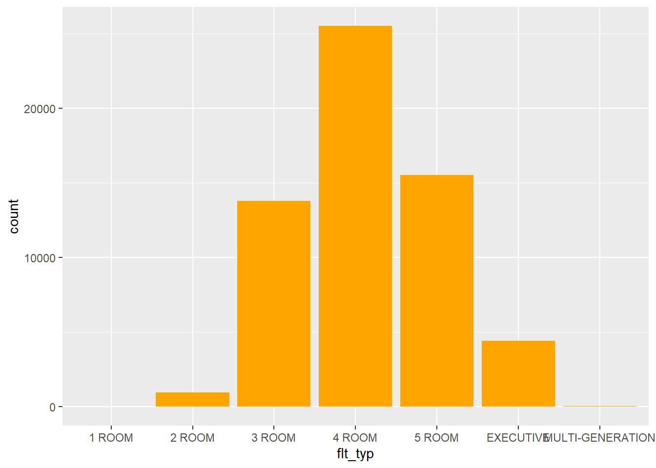
Looks like 4-room apartments have the most transactions. Whereas 5-room and 3-room flats come second and third respectively. There could be more interest in these sort of flats, but can also be due to most flats are 3 to 5 room flats, which limits options available.
8 Preparation for Modelling
We will now move on to model preparation.
8.1 Filtering
8.1.1 Train
Sadly due to my laptop’s limited computation power, I have filtered the training data to be only from June 2022 to December 2022 :(
We will also filter for the columns that are of interest to us, as shown below.
 [1] "floor_area_sqm"    "resale_price"      "HIP"
 [4] "MUP"               "PROX_CBD"          "PROX_HAWKER"
 [7] "PROX_ELDERCARE"    "PROX_KINDERGARTEN" "PROX_CHILDCARE"
[10] "PROX_BUSSTOP"      "PROX_MRT"          "PROX_SCH"
[13] "PROX_SUPERMARKET"  "PROX_MALL"         "PROX_TOPSCH"
[16] "NUM_KINDERGARTEN"  "NUM_CHILDCARE"     "NUM_BUSSTOP"
[19] "NUM_SCH"           "NUM_TOPSCH"        "storey_names"
[22] "remaining_lease" "age" 8.1.2 Test
The test data is then this year’s transactions, being in January and February 2023.
8.2 Visualising the relationships of the independent variables
We will want to check for multicollinearity, in that whether any of the variables is highly correlated with one another. If not removed, the models may not be wholy representative of the different variables and the predicted hence then be wrong.
Correlation matrix is what we will be using in this section.
corrplot(cor(total_resale_prices), diag = FALSE, order = "AOE",
         tl.pos = "td", tl.cex = 0.5, method = "number", type = "upper")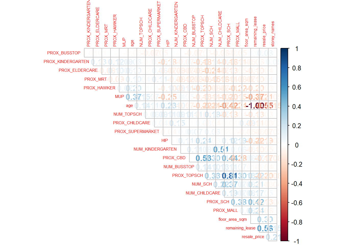
Looks like age of the HDB flats and remaining lease are practically inversely correlated, having a correlation of more than +/-0.8. So one will be removed, age will be removed.
Similarly, proximity of schools will be removed in favour of top schools.
9 OLS Multiple Linear Regression (MLR) Model
lm() is applied to calibrate our MLR model.
resale_price.mlr <- lm(formula = resale_price ~ floor_area_sqm + HIP + MUP + PROX_CBD + PROX_HAWKER +  PROX_ELDERCARE + PROX_KINDERGARTEN + PROX_CHILDCARE + PROX_BUSSTOP + PROX_MRT +  PROX_SUPERMARKET + PROX_MALL + PROX_TOPSCH + NUM_KINDERGARTEN + NUM_CHILDCARE + NUM_BUSSTOP + NUM_TOPSCH, data = train_resale_prices)
summary(resale_price.mlr)
Call:
lm(formula = resale_price ~ floor_area_sqm + HIP + MUP + PROX_CBD +
    PROX_HAWKER + PROX_ELDERCARE + PROX_KINDERGARTEN + PROX_CHILDCARE +
    PROX_BUSSTOP + PROX_MRT + PROX_SUPERMARKET + PROX_MALL +
    PROX_TOPSCH + NUM_KINDERGARTEN + NUM_CHILDCARE + NUM_BUSSTOP +
    NUM_TOPSCH, data = train_resale_prices)

Residuals:
    Min      1Q  Median      3Q     Max
-197750  -44066   -7648   25846  374913

Coefficients:
                    Estimate Std. Error t value Pr(>|t|)
(Intercept)         218087.4    17354.7  12.566  < 2e-16 ***
floor_area_sqm        4323.4      215.9  20.025  < 2e-16 ***
HIP                 -49268.5     3056.3 -16.120  < 2e-16 ***
MUP                 -71581.5     3522.0 -20.324  < 2e-16 ***
PROX_CBD          -1353368.7   470396.3  -2.877 0.004036 **
PROX_HAWKER        -203613.4    32186.0  -6.326 2.81e-10 ***
PROX_ELDERCARE      -64468.8    33981.1  -1.897 0.057879 .
PROX_KINDERGARTEN    11029.0     8914.9   1.237 0.216113
PROX_CHILDCARE       -2824.4     2547.1  -1.109 0.267562
PROX_BUSSTOP          3176.9      803.2   3.955 7.79e-05 ***
PROX_MRT            -33628.6    20361.6  -1.652 0.098707 .
PROX_SUPERMARKET    -47490.5     8602.1  -5.521 3.60e-08 ***
PROX_MALL          -186034.1    37614.8  -4.946 7.92e-07 ***
PROX_TOPSCH       -3018241.6   318717.7  -9.470  < 2e-16 ***
NUM_KINDERGARTEN     -6320.2     1667.9  -3.789 0.000153 ***
NUM_CHILDCARE         2240.5      762.8   2.937 0.003332 **
NUM_BUSSTOP           -590.6      484.9  -1.218 0.223333
NUM_TOPSCH           10060.3     2620.8   3.839 0.000126 ***
---
Signif. codes:  0 '***' 0.001 '**' 0.01 '*' 0.05 '.' 0.1 ' ' 1

Residual standard error: 73950 on 3741 degrees of freedom
Multiple R-squared:  0.2777,    Adjusted R-squared:  0.2744
F-statistic: 84.61 on 17 and 3741 DF,  p-value: < 2.2e-16
9.1 Preparation of Publication Quality Table
Using tbl_regression(), we want to find out which variables are not significant significant enough to retain in the model.
| Characteristic | Beta | 95% CI1 | p-value |
|---|---|---|---|
| (Intercept) | 218,087 | 184,062, 252,113 | <0.001 |
| floor_area_sqm | 4,323 | 3,900, 4,747 | <0.001 |
| HIP | -49,268 | -55,261, -43,276 | <0.001 |
| MUP | -71,581 | -78,487, -64,676 | <0.001 |
| PROX_CBD | -1,353,369 | -2,275,627, -431,111 | 0.004 |
| PROX_HAWKER | -203,613 | -266,717, -140,510 | <0.001 |
| PROX_ELDERCARE | -64,469 | -131,092, 2,154 | 0.058 |
| PROX_KINDERGARTEN | 11,029 | -6,450, 28,508 | 0.2 |
| PROX_CHILDCARE | -2,824 | -7,818, 2,169 | 0.3 |
| PROX_BUSSTOP | 3,177 | 1,602, 4,752 | <0.001 |
| PROX_MRT | -33,629 | -73,550, 6,292 | 0.10 |
| PROX_SUPERMARKET | -47,490 | -64,356, -30,625 | <0.001 |
| PROX_MALL | -186,034 | -259,782, -112,287 | <0.001 |
| PROX_TOPSCH | -3,018,242 | -3,643,119, -2,393,364 | <0.001 |
| NUM_KINDERGARTEN | -6,320 | -9,590, -3,050 | <0.001 |
| NUM_CHILDCARE | 2,241 | 745, 3,736 | 0.003 |
| NUM_BUSSTOP | -591 | -1,541, 360 | 0.2 |
| NUM_TOPSCH | 10,060 | 4,922, 15,199 | <0.001 |
| 1 CI = Confidence Interval | |||
With PROX_ELDERCARE, PROX_KINDERGARTEN, PROX_CHILDCARE, PROX_MRT and NUM_BUSSTOP having a p-value above 0.01, we will subsequently remove them to improve our model.
| Characteristic | Beta | 95% CI1 | p-value |
|---|---|---|---|
| (Intercept) | 202,017 | 171,060, 232,974 | <0.001 |
| floor_area_sqm | 4,341 | 3,919, 4,762 | <0.001 |
| HIP | -49,680 | -55,614, -43,746 | <0.001 |
| MUP | -71,982 | -78,869, -65,095 | <0.001 |
| PROX_CBD | -1,094,917 | -1,992,630, -197,205 | 0.017 |
| PROX_HAWKER | -200,882 | -263,045, -138,720 | <0.001 |
| PROX_BUSSTOP | 3,285 | 1,713, 4,857 | <0.001 |
| PROX_SUPERMARKET | -50,517 | -67,150, -33,883 | <0.001 |
| PROX_MALL | -172,911 | -245,285, -100,536 | <0.001 |
| PROX_TOPSCH | -3,177,094 | -3,784,479, -2,569,709 | <0.001 |
| NUM_KINDERGARTEN | -6,478 | -9,669, -3,287 | <0.001 |
| NUM_CHILDCARE | 2,428 | 955, 3,901 | 0.001 |
| NUM_TOPSCH | 9,496 | 4,394, 14,598 | <0.001 |
| 1 CI = Confidence Interval | |||
9.2 Save to RDS
9.3 Read RDS
Call:
lm(formula = resale_price ~ floor_area_sqm + HIP + MUP + PROX_CBD +
    PROX_HAWKER + +PROX_BUSSTOP + PROX_SUPERMARKET + PROX_MALL +
    PROX_TOPSCH + NUM_KINDERGARTEN + NUM_CHILDCARE + NUM_TOPSCH,
    data = train_resale_prices)

Residuals:
    Min      1Q  Median      3Q     Max
-204779  -44453   -7564   25831  378838

Coefficients:
                   Estimate Std. Error t value Pr(>|t|)
(Intercept)        202017.3    15789.7  12.794  < 2e-16 ***
floor_area_sqm       4340.5      214.8  20.210  < 2e-16 ***
HIP                -49679.5     3026.6 -16.414  < 2e-16 ***
MUP                -71981.8     3512.6 -20.492  < 2e-16 ***
PROX_CBD         -1094917.1   457877.0  -2.391 0.016838 *
PROX_HAWKER       -200882.5    31705.8  -6.336 2.64e-10 ***
PROX_BUSSTOP         3284.7      801.8   4.096 4.28e-05 ***
PROX_SUPERMARKET   -50516.8     8483.9  -5.954 2.85e-09 ***
PROX_MALL         -172910.5    36914.5  -4.684 2.91e-06 ***
PROX_TOPSCH      -3177094.1   309795.9 -10.255  < 2e-16 ***
NUM_KINDERGARTEN    -6478.0     1627.5  -3.980 7.01e-05 ***
NUM_CHILDCARE        2428.2      751.3   3.232 0.001240 **
NUM_TOPSCH           9496.4     2602.3   3.649 0.000267 ***
---
Signif. codes:  0 '***' 0.001 '**' 0.01 '*' 0.05 '.' 0.1 ' ' 1

Residual standard error: 73990 on 3746 degrees of freedom
Multiple R-squared:  0.276, Adjusted R-squared:  0.2737
F-statistic:   119 on 12 and 3746 DF,  p-value: < 2.2e-16
:::
Yes! Now, there are no more insignificant variables. Let’s move on.
9.4 Checking for Non-Linearity
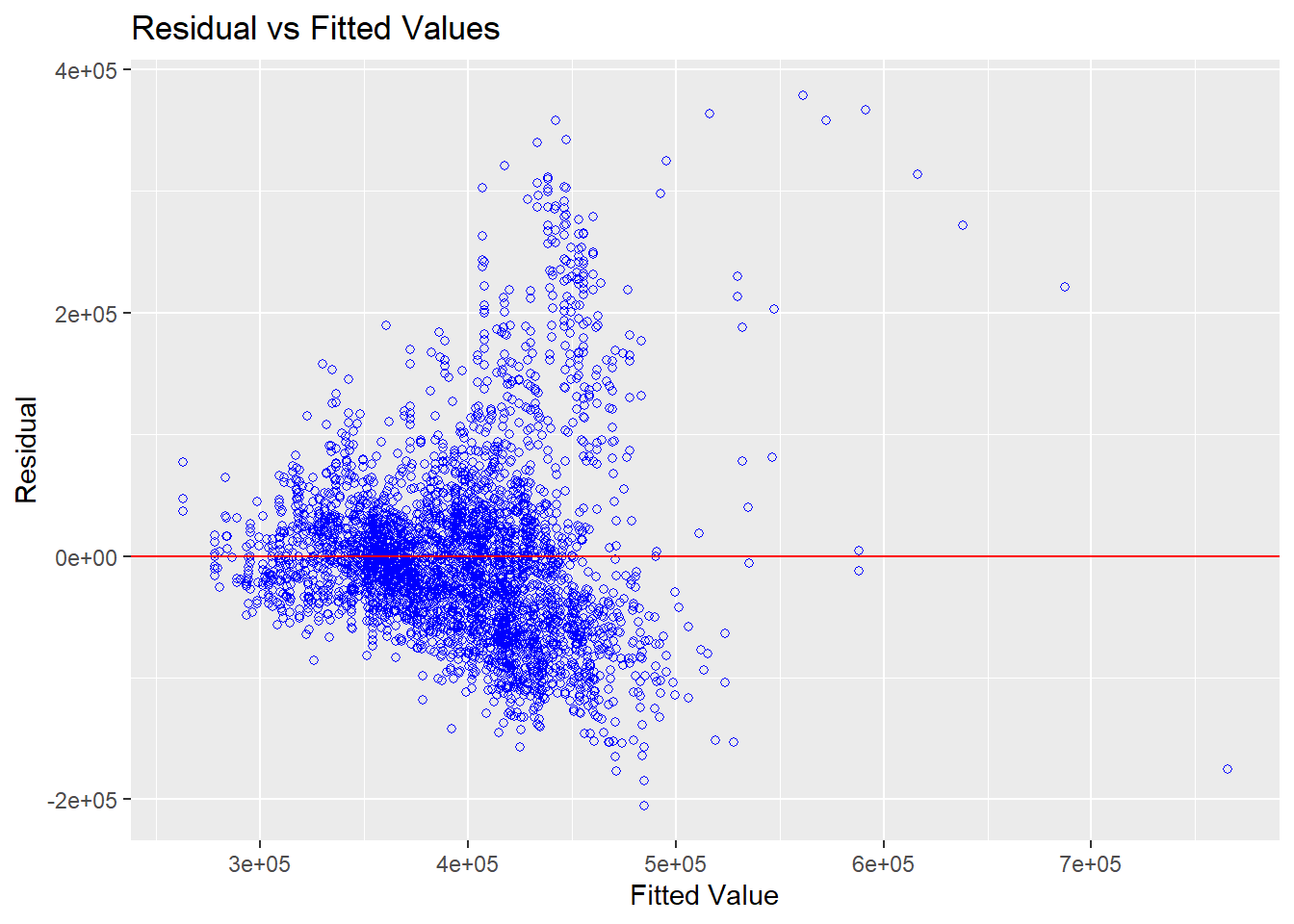
With most datapoints scatter on and around the 0 line, we can determine the relationship is linear.
9.5 Checking for Normality Assumption
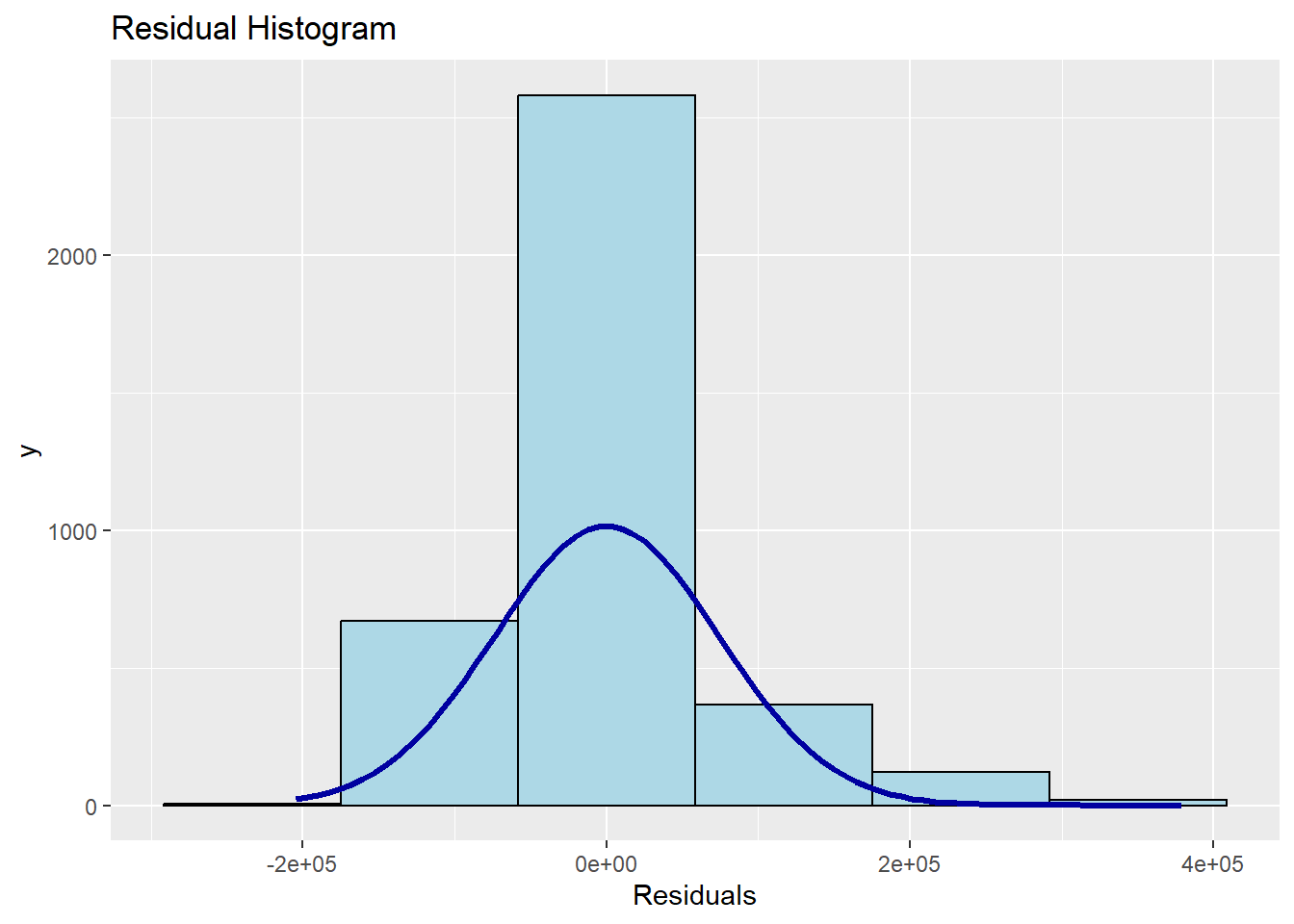
The model is also normal in distribution.
9.6 Checking for Spatial Autocorrelation
With this test, we then check for the spatial variation in resell prices using the residuals from our MLR model.
Because we need the geospatial polygons to map our residuals and that spdep package only processes sp datatype, we will first convert resale_price.mlr to a DataFrame, then to a sf DataFrame, finally a sp DataFrame.
resale_price.mlr.output <- as.data.frame(resale_price.mlr$residuals)
final_resale_price.mlr.sf <- cbind(train_resale_prices, resale_price.mlr.output) %>%
  rename(`MLR_RES` = `resale_price.mlr.residuals`)
final_resale_price.mlr.sp <- as_Spatial(final_resale_price.mlr.sf)
final_resale_price.mlr.sp
class : SpatialPointsDataFrame
features : 3759
extent : 11597.97, 45154.27, 28097.64, 48622.47 (xmin, xmax, ymin, ymax)
crs : +proj=tmerc +lat_0=1.36666666666667 +lon_0=103.833333333333 +k=1 +x_0=28001.642 +y_0=38744.572 +ellps=WGS84 +towgs84=0,0,0,0,0,0,0 +units=m +no_defs
variables : 24
names : floor_area_sqm, resale_price, HIP, MUP, PROX_CBD, PROX_HAWKER, PROX_ELDERCARE, PROX_KINDERGARTEN, PROX_CHILDCARE, PROX_BUSSTOP, PROX_MRT, PROX_SCH, PROX_SUPERMARKET, PROX_MALL, PROX_TOPSCH, ...
min values : 51, 240000, 0, 0, 0.001, 0.002, 0.001, 0.001, 0.002, 0.005, 0.001, 0.001, 0.001, 0.003, 0.001, ...
max values : 137, 958000, 1, 1, 0.013, 0.125, 0.133, 0.438, 1.912, 5.138, 0.217, 0.181, 0.526, 0.167, 0.02, ... 9.6.1 Visualisation
tmap_mode("view")
tm_shape(subzone_sf)+
  tmap_options(check.and.fix = TRUE) +
  tm_polygons(alpha = 0.4) +
tm_shape(final_resale_price.mlr.sf) +
  tm_dots(col = "MLR_RES",
          alpha = 0.6,
          style="quantile") +
tm_view(set.zoom.limits = c(11,14))From the visualisation, we can determine that there are signs of spatial autocorrelation.
9.7 Prediction
Finally, we come to prediction.
Using Root Mean Square Error (RMSE), we can observe the difference between the predicted values and the actual values, which enables us to determine whether the model fares well in predicting.
9.7.1 Visualisation
ols_scatterplot <- ggplot(data = test_data_mlr,
       aes(x = mlr_pred,
           y = resale_price)) +
  geom_point() +
  geom_abline(col = "Red")

ols_scatterplot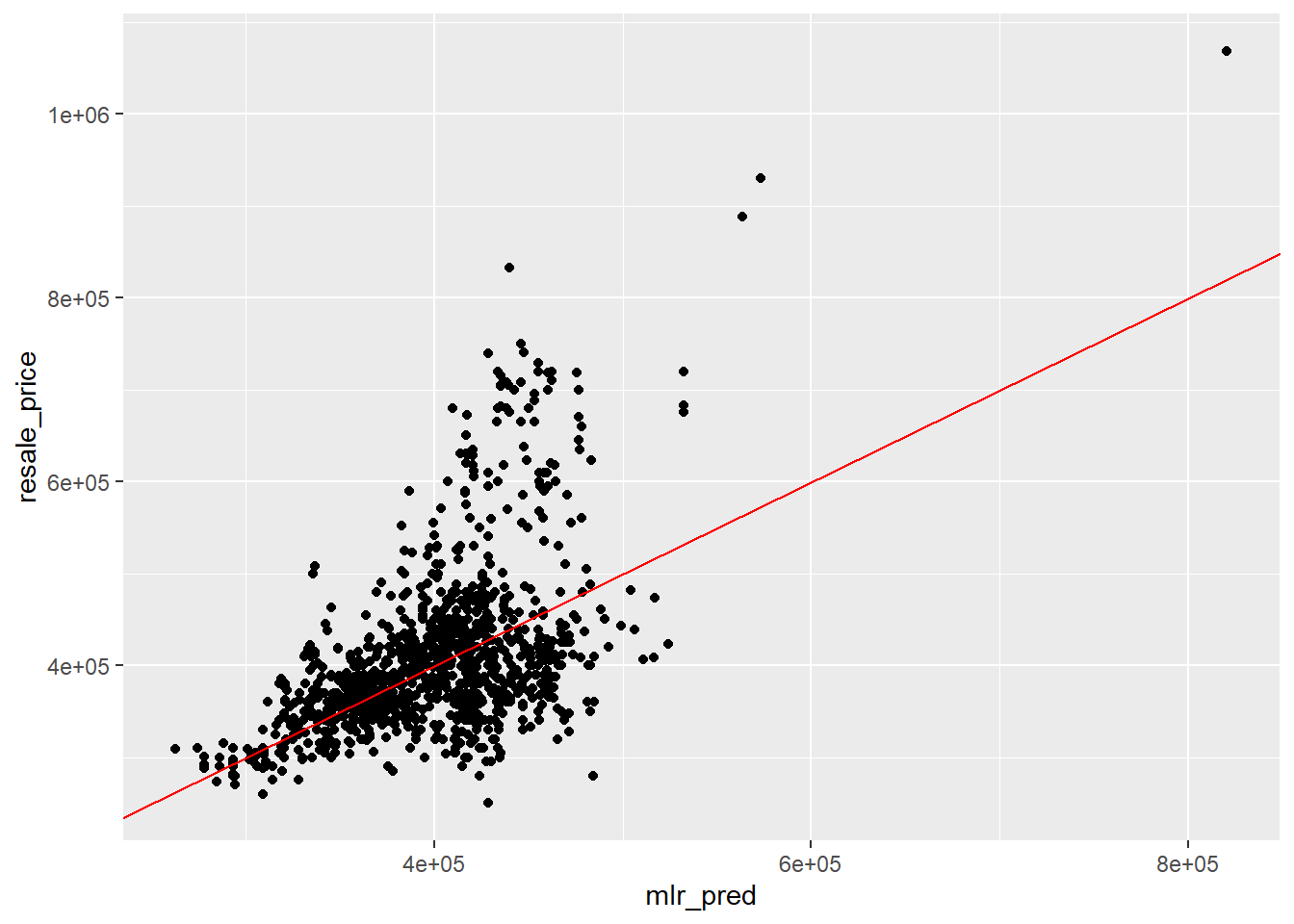
Although there is a visible trend in how the datapoints are structured (i.e., a line), you can see that most datapoints fall out this line. This suggests that the model is probably decent, but has way more areas for improvements in order to accurately predict future transactional prices.
10 Geographical Random Forest Model (GRFW)
In this section, we are seeking to create a GRFM through an adaptive bandwidth approach
Since conducting the Random Forest model will require us to drop the coordinates, we will first save them.
10.1 Optimal Bandwidth
Since we are creating an adaptive model, we will use bw.gwr() from GWmodel package to determine the optimal bandwidth.
set.seed(1234)
bw_adaptive <- bw.gwr(resale_price ~ floor_area_sqm + HIP + MUP + PROX_CBD + PROX_HAWKER +  PROX_ELDERCARE + PROX_KINDERGARTEN + PROX_CHILDCARE + PROX_BUSSTOP + PROX_MRT +  PROX_SUPERMARKET + PROX_MALL + PROX_TOPSCH + NUM_KINDERGARTEN + NUM_CHILDCARE + NUM_BUSSTOP + NUM_TOPSCH,
                      data=resale_price.sp,
                      approach="CV",
                      kernel="gaussian",
                      adaptive=TRUE,
                      longlat=FALSE)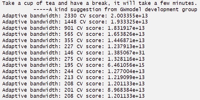
As you can see from above, the most suitable bandwidth is 208.
10.2 Calibration of Geographical Random Forest Model (GRFM)
Using the SpatialML package, we calibrate our Random Forest model from there.
set.seed(1234)
grf_adaptive <- grf(formula = resale_price ~ floor_area_sqm + HIP + MUP + PROX_CBD + PROX_HAWKER +  PROX_ELDERCARE + PROX_KINDERGARTEN + PROX_CHILDCARE + PROX_SUPERMARKET + PROX_MALL + PROX_TOPSCH + NUM_KINDERGARTEN + NUM_CHILDCARE + NUM_BUSSTOP + NUM_SCH + NUM_TOPSCH,
                     dframe=train_resale_prices,
                     bw=bw_adaptive,
                     kernel="adaptive",
                     coords=coords_train,
ntree = 30)10.3 Prediction
10.3.1 Preparation
Now, we can combine the test data and coordinates together.
And onwards to our prediction using predict.grf() using the above variable.
10.3.1.1 Visualisation
Like in the OLS model above, we will use calculate the RMSE to determine the accuracy of our new model.
ggplot(data = test_data_plot,
       aes(x = gwRF_pred,
           y = resale_price)) +
  geom_point() +
  geom_abline(col = "Red")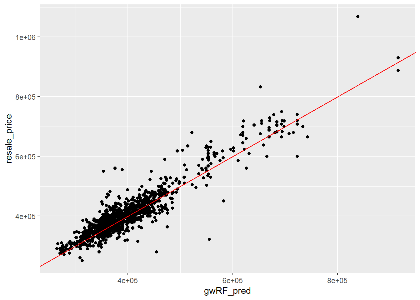
The chart showcases the datapoints scattered relatively straight across a line, suggesting predicted resale prices and actual resale prices are quite close together.
11 Conclusion
In comparing the two different models, the Geographical Random Forest model perform way better than Linear Regression using OSL method, in predicting resell prices for 3-room flats. This is in line with what we know with how Linear Regression fails to take into account with some geospatial conditions like spatial autocorrelation.
Interesting, we eliminated childcare centres, kindergartens and proxity to MRT due to them not being significant enough to be included in the Multi-Linear Regression model, which is shocking personally. In the context of this exercise, it is not known whether there is a difference in significant variables among different flat types (e.g., 2-room). Personally, I may suspect that this is due to the diverse demographics (particularly singles) that purchase this sort of flat type, in contrast with other types.
12 Acknowledges
Professor Kam Tin Seong’s Exercises: